Primate activity pattern and orbit morphology: a phylogenetic analysis of data from Kirk & Kay (2004)
17 Nov 2017Previous studies have found a strong association between nocturnal activity patterns and orbit size across primates (Walker 1967; Cartmill 1970; Kay & Cartmill 1977; Martin 1990; Kay & Kirk 2000). This association is thought to reflect adaptations to the visual system in nocturnal primates, since larger eyeballs enhance visual sensitivity. Kay & Kirk (2000) also found a highly signficant negative correlation between nocturnality and a small optic foramen relative to the size of the orbit, which is argued to be an adaptation for greater retinal summation in nocturnal primates. However, these studies failed to account for phylogenetic non-independence in their analyses, which can increase the risk ot Type 1 error (Felsenstein 1985).
In this post, I revisit the relationship between activity pattern and orbit/optic foramen size in primates using phylogenetic generalized least squares (PGLS), which accounts for phylogeny in the variance-covariance structure of linear models (Martins & Hansen 1997). I also fit OLS models for comparison to the PGLS models. Rather than reanalyzing data the 60-taxa dataset from Kay & Kirk (2000), I instead analyze the expanded and improved dataset on skull length, orbit size, and optic foramen size provided more recently by Kirk & Kay (2004), which includes more accurate esimates of species means, 33 additional species for a total of n = 93, and computes orbit area from orbit diameter in a more realistic way by assuming the orbit is circular rather than square (an odd assumption made by Kay & Kirk 2000). I dropped 3 species from the dataset due to lack of phylogenetic data, yielding a total of n = 90 taxa.
I’m happy to say that my PGLS analyses produce the same inferences made by Kay & Kirk (2000): both orbit size and relative optic foramen size are significantly associated with activity pattern after controlling for skull length. However, there is severe phylogenetic non-independence in both models, and the strength of statistical support is drastically reduced when PGLS is used instead of OLS. To replicate my analysis in R, load the following packages and import the data from my website (the phylogeny comes from 10kTrees):
# load packages
library("caper")
library("ggplot2")

# import data
data <- read.csv("/Users/nunnlab/Desktop/GitHub/rgriff23.github.io/assets/data/kaykirk2004.csv")
tree <- readRDS("/Users/nunnlab/Desktop/GitHub/rgriff23.github.io/assets/Rds/kaykirk2004_tree.Rds")
The dataset includes the following variables:
Genus_species- Genus and species nameGroup- Prosimian or AnthropoidSkull_length- Prosthion-inion linear distance in mmOptic_foramen_area- Optic forament area in square mmOrbit_area- Orbit area in square mm, estimated from orbit diameterActivity_pattern- Diurnal, cathemeral, or nocturnalActivity_pattern_code- 0 = Diurnal, 1 = Cathemeral, and 2 = Nocturnal
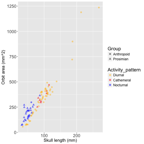
Below is a scatterplot of orbit size against skull length, with data points colored based on activity pattern. Prosimians are represented by triangles and anthropoids by circles to show the strong phylogenetic pattern in the data. This plot also displays the allometry of orbit size, which is why it is important to control for skull length in analyses of orbit size:
# create factor levels for activiy pattern (ensures desired ordering in plot legend)
data$Activity_pattern <- factor(data$Activity_pattern, levels=c("Diurnal","Cathemeral","Nocturnal"))

# scatterplot of orbit diameter against skull length
ggplot(data, aes(Skull_length, Orbit_area, color=Activity_pattern, shape=Group)) +
  geom_point(alpha=0.5, size=2.5) +
  scale_color_manual(values=c("goldenrod1","red","blue")) +
  xlab("Skull length (mm)") +
  ylab("Orbit area (mm^2)") +
  theme(axis.text=element_text(size=15),
        axis.title=element_text(size=15),
        legend.text=element_text(size=12),
        legend.title=element_text(size=17))

This plot illustrates the challenge of disentangling the association between orbit size and activity pattern from the effects of phylogenetic history - most of the nocturnal species are prosimians (blue triangles), and most of the diurnal species are anthropoids (yellow circles). Let’s fit an OLS model to the data, controlling for skull length by including it as a covariate:
# OLS: orbit diameter ~ nocturnal + log body size
mod1 <- lm(Orbit_area ~ Activity_pattern_code + Skull_length, data=data)
summary(mod1)
>
>  Call:
>  lm(formula = Orbit_area ~ Activity_pattern_code + Skull_length,
>      data = data)
>
>  Residuals:
>      Min      1Q  Median      3Q     Max
>  -99.658 -33.601  -4.527  27.488 228.884
>
>  Coefficients:
>                         Estimate Std. Error t value Pr(>|t|)
>  (Intercept)           -158.1029    17.4092  -9.082 3.06e-14 ***
>  Activity_pattern_code   41.4516     7.0501   5.880 7.44e-08 ***
>  Skull_length             5.2376     0.1613  32.462  < 2e-16 ***
>  ---
>  Signif. codes:  0 '***' 0.001 '**' 0.01 '*' 0.05 '.' 0.1 ' ' 1
>
>  Residual standard error: 51.8 on 87 degrees of freedom
>  Multiple R-squared:  0.9337,	Adjusted R-squared:  0.9322
>  F-statistic: 612.7 on 2 and 87 DF,  p-value: < 2.2e-16
Results show that relative orbit size is strongly associated with activity pattern (p = 0.0000000744). Now let’s fit a PGLS model to the same data. I allow the model to estimate the phylogenetic signal parameter ‘lambda’ by specifying lambda="ML". Lambda = 0 if there is no phylogenetic non-independence in the model residuals, and lambda = 1 if the phylogeny provides a good description of the model residuals (Pagel 1999).
# PGLS: orbit circumference ~ nocturnal + log body size
comp.dat = comparative.data(tree, data, names.col="Genus_species")
mod2 <- pgls(Orbit_area ~ Activity_pattern_code + Skull_length, data=comp.dat, lambda="ML")
summary(mod2)
>
>  Call:
>  pgls(formula = Orbit_area ~ Activity_pattern_code + Skull_length,
>      data = comp.dat, lambda = "ML")
>
>  Residuals:
>      Min      1Q  Median      3Q     Max
>  -24.571  -6.911  -0.111   7.377  44.244
>
>  Branch length transformations:
>
>  kappa  [Fix]  : 1.000
>  lambda [ ML]  : 1.000
>     lower bound : 0.000, p = 0.00019742
>     upper bound : 1.000, p = 1
>     95.0% CI   : (0.749, NA)
>  delta  [Fix]  : 1.000
>
>  Coefficients:
>                          Estimate Std. Error t value Pr(>|t|)
>  (Intercept)           -117.07443   52.51626 -2.2293  0.02837 *
>  Activity_pattern_code   35.63624   14.69841  2.4245  0.01740 *
>  Skull_length             5.08396    0.26484 19.1961  < 2e-16 ***
>  ---
>  Signif. codes:  0 '***' 0.001 '**' 0.01 '*' 0.05 '.' 0.1 ' ' 1
>
>  Residual standard error: 12.15 on 87 degrees of freedom
>  Multiple R-squared: 0.8095,	Adjusted R-squared: 0.8051
>  F-statistic: 184.8 on 2 and 87 DF,  p-value: < 2.2e-16
The maximum likelihood estimate of lambda is 1, indicating a high degree of phylogenetic non-independence, and the relationship between orbit area and activity pattern is now barely statistically significant (p = 0.017). This demonstrates that the data are strongly structured by phylogenetic relationships and that standard errors were greatly underestimated when OLS was used.
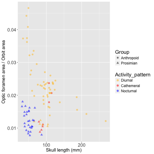
Now let’s compare OLS and PGLS results for relative optic foramen area, beginning with a visualization the relationship between relative optic foramen area versus skull length:
# scatterplot of relative optic foramen area against skull length
ggplot(data, aes(Skull_length, Optic_foramen_area/Orbit_area, color=Activity_pattern, shape=Group)) +
  geom_point(alpha=0.5, size=2.5) +
  scale_color_manual(values=c("goldenrod1","red","blue")) +
  xlab("Skull length (mm)") +
  ylab("Optic foramen area / Orbit area") +
  theme(axis.text=element_text(size=15),
        axis.title=element_text(size=15),
        legend.text=element_text(size=12),
        legend.title=element_text(size=17))

We can see that the separation between nocturnal prosimians (blue triangles) and diurnal anthropoids (yellow circles) is even more extreme for relative optic foramen size than for orbit area. Let’s fit an OLS model to this data:
# OLS: relative optic foramen size ~ nocturnal + log body size
mod3 <- lm((Optic_foramen_area/Orbit_area) ~ Activity_pattern_code + Skull_length, data=data)
summary(mod3)
>
>  Call:
>  lm(formula = (Optic_foramen_area/Orbit_area) ~ Activity_pattern_code +
>      Skull_length, data = data)
>
>  Residuals:
>         Min         1Q     Median         3Q        Max
>  -0.0143145 -0.0032917 -0.0001434  0.0034086  0.0185568
>
>  Coefficients:
>                          Estimate Std. Error t value Pr(>|t|)
>  (Intercept)            3.331e-02  1.994e-03  16.700  < 2e-16 ***
>  Activity_pattern_code -7.853e-03  8.077e-04  -9.723 1.49e-15 ***
>  Skull_length          -1.071e-04  1.848e-05  -5.795 1.07e-07 ***
>  ---
>  Signif. codes:  0 '***' 0.001 '**' 0.01 '*' 0.05 '.' 0.1 ' ' 1
>
>  Residual standard error: 0.005934 on 87 degrees of freedom
>  Multiple R-squared:  0.5225,	Adjusted R-squared:  0.5115
>  F-statistic:  47.6 on 2 and 87 DF,  p-value: 1.086e-14
This model finds extremely strong evidence for a link between relative optic foramen area and activity pattern (p = 0.00000000000000149). But if we fit a PGLS model:
# PGLS: relative optic foramen size ~ nocturnal + log body size
mod4 <- pgls((Optic_foramen_area/Orbit_area) ~ Activity_pattern_code + Skull_length, data=comp.dat, lambda="ML")
summary(mod4)
>
>  Call:
>  pgls(formula = (Optic_foramen_area/Orbit_area) ~ Activity_pattern_code +
>      Skull_length, data = comp.dat, lambda = "ML")
>
>  Residuals:
>         Min         1Q     Median         3Q        Max
>  -0.0026004 -0.0006721 -0.0001027  0.0004033  0.0027738
>
>  Branch length transformations:
>
>  kappa  [Fix]  : 1.000
>  lambda [ ML]  : 0.958
>     lower bound : 0.000, p = 5.5511e-15
>     upper bound : 1.000, p = 0.0095447
>     95.0% CI   : (0.853, 0.995)
>  delta  [Fix]  : 1.000
>
>  Coefficients:
>                           Estimate  Std. Error t value  Pr(>|t|)
>  (Intercept)            2.6059e-02  4.0581e-03  6.4216 6.887e-09 ***
>  Activity_pattern_code -4.0176e-03  1.1809e-03 -3.4022 0.0010119 **
>  Skull_length          -8.8506e-05  2.1829e-05 -4.0546 0.0001091 ***
>  ---
>  Signif. codes:  0 '***' 0.001 '**' 0.01 '*' 0.05 '.' 0.1 ' ' 1
>
>  Residual standard error: 0.0009302 on 87 degrees of freedom
>  Multiple R-squared: 0.2125,	Adjusted R-squared: 0.1944
>  F-statistic: 11.74 on 2 and 87 DF,  p-value: 3.067e-05
The maximum likelihood estimate of lambda is very close to 1, and the relationship between relative optic foramen size and activity pattern is drastically weakened, although still highly significant (p = 0.001). This suggests that relative optic foramen size may be a more reliable indicator of activity pattern than relative orbit size.
These results uphold the conclusions of Kay & Kirk (2000) while simultaneously illustrating the statistical importance of accounting for autocorrelated data in regression models. In particular, despite the striking visual pattern in the data, the relationship between orbit size and activity pattern is barely significant when phylogenetic relationships are incorporated into the model.
Footnote: Although I don’t report it here, I have found that the link between activity pattern and orbit size is not statistically significant when the original 60-taxa dataset from Kay & Kirk (2000) is analyzed with PGLS rather than OLS. In fact, that is what inspired me to analyze the improved dataset from Kirk & Kay (2004). Since the conclusions of Kay & Kirk (2000) are upheld when the superior dataset is used, I decided to stay focused on that.
References
Cartmill M. 1970. The orbits of arboreal mammals: a reassessment of the arboreal theory of primate evolution. Ph.D. dissertation. Chicago: University of Chicago.
Felsenstein J. 1985. Phylogenies and the comparative method. The American Naturalist, 125(1), pp.1-15.
Kay RF, Cartmill M. 1977. Cranial morphology and adaptation of Palaechthon nacimienti and other Paromomyidae (Plesiadapoidea ?Primates), with a description of a new genus and species. J Hum Evol 6:19-35.
Kay RF, Kirk EC. 2000. Osteological evidence for the evolution of activity pattern and visual acuity in primates. American Journal of Physical Anthropology, 113(2), pp.235-262.
Kirk EC, Kay RF. 2004. The evolution of high visual acuity in the Anthropoidea. In Anthropoid Origins (pp. 539-602). Springer US.
Martins EP, Hansen TF. 1997. Phylogenies and the comparative method: a general approach to incorporating phylogenetic information into the analysis of interspecific data. Am Nat 149:646–667.
Pagel M. 1999. Inferring the historical patterns of biological evolution. Nature, 401(6756), p.877.
Walker A. 1967. Patterns of extinction among subfossil Madagascan lemuroids. In: Martin PS, Wright HE (Eds). Pleistocene extinctions: the search for a cause. New Haven: Yale University Press.
